In quantum mechanics, particles are represented by ‘wave functions’, wavy entities that are extended in space. The square modulus of the wave at any location gives the probability density of finding the particle at that location. The behavior of the waves is given by the time-dependent Schrödinger equation – a wave equation that describes how the waves evolve in time.
Interpreting quantum mechanics is a notoriously abstract and subtle business; much discussion exists regarding the ontological status of the waves, as well as their connection to the point-like particles we observe in actual experiments – we never observe waves, only particles (this is related to the so-called ‘measurement problem’). We won’t look at measurements in this series of posts – instead we will only consider the time evolution of quantum mechanical systems while they are not measured. This evolution is wave-like and fully deterministic, and it can be readily visualized, which may help us to understand it more intuitively.
We can do this by concocting an initial wave configuration and then solving the wave equation using a computer, plotting the evolving wave at each moment in time. Stitching the resulting plots together into an animation then yields a visual picture of the quantum mechanical process we are examining.
In this series of posts, I will describe and publish the C++ code I have developed for this purpose. In this first entry I’ll have an introductory look at solving the time-dependent Schrödinger equation (TDSE), which determines the time evolution of an initial wave function 
Mathematical description of a one-particle system
The TDSE reads as follows:
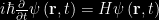
where 


![i\hbar \frac{\partial}{\partial t} \psi = \left[-\frac{\hbar}{2m} {\nabla}^2 + V \right] \psi](https://s0.wp.com/latex.php?latex=i%5Chbar+%5Cfrac%7B%5Cpartial%7D%7B%5Cpartial+t%7D+%5Cpsi+%3D+%5Cleft%5B-%5Cfrac%7B%5Chbar%7D%7B2m%7D+%7B%5Cnabla%7D%5E2+%2B+V+%5Cright%5D+%5Cpsi&bg=000000&fg=ffffff&s=0&c=20201002)
where 
- The particle’s initial wave function,
.
- The potential in which the particle finds itself,
Equation (1) itself can then be discretized and solved numerically, for example by using a simple Euler scheme:
![\psi_{n+1} = \psi_{n} + \frac{\Delta t}{i \hbar} \left[-\frac{\hbar}{2m} {\nabla}^2 + V \right] \psi_{n}\\ t_{n+1}=t_n+\Delta t.](https://s0.wp.com/latex.php?latex=%5Cpsi_%7Bn%2B1%7D+%3D+%5Cpsi_%7Bn%7D+%2B+%5Cfrac%7B%5CDelta+t%7D%7Bi+%5Chbar%7D+%5Cleft%5B-%5Cfrac%7B%5Chbar%7D%7B2m%7D+%7B%5Cnabla%7D%5E2+%2B+V+%5Cright%5D+%5Cpsi_%7Bn%7D%5C%5C++t_%7Bn%2B1%7D%3Dt_n%2B%5CDelta+t.&bg=000000&fg=ffffff&s=0&c=20201002)
Thus, to evolve the wave function in time, we act on it with the operator ![\left[-\frac{\hbar}{2m} {\nabla}^2 + V \right]](https://s0.wp.com/latex.php?latex=%5Cleft%5B-%5Cfrac%7B%5Chbar%7D%7B2m%7D+%7B%5Cnabla%7D%5E2+%2B+V+%5Cright%5D+&bg=000000&fg=ffffff&s=0&c=20201002)

Some examples
I. A coherent state of the quantum harmonic oscillator
As a first example, let’s look at the time evolution of a coherent state of the harmonic oscillator (for a refresher on coherent states, see this University of Virginia page). The initial wave function is a Gaussian packet that is displaced from the center of the potential and centered at 
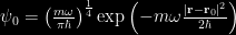
where 

Plugging these expressions into equation (1) and solving that equation numerically yields the time evolution of the coherent state. After each time step, we plot the wave function; finally we create an animation by playing the plots in sequence.
The wave function assigns a complex number (probability amplitude) to each point in space. We’ll plot the wave function as follows; the hue of each pixel represents the complex phase, while the intensity represents the complex amplitude. The potential, meanwhile, is plotted in white (the higher the potential, the brighter the pixel).
Let’s look at the result:
As you can see, the wave packet of the coherent state retains its exact shape indefinitely – only its phase changes. It is the closest thing in quantum mechanics to a classical particle oscillating back and forth.
II. The double-slit experiment
The coherent state and its temporal evolution have actually been solved analytically. A more interesting example, which is impossible to solve analytically, is the famous double-slit experiment. To recreate it numerically, let’s construct a suitable wave function; we want it to be localized (suggesting a Gaussian packet once again) as well as in a state of motion toward the two slits. To accomplish this we will modulate the Gaussian packet’s complex phase, giving it a non-zero momentum:
![\psi_0=\exp{\left(-\frac{\left| {\bf r} - {\bf r_0}\right|^2}{2\sigma^2}\right)} \left[\sin{\left( x k\right)}+i \cos{\left(x k \right)}\right]](https://s0.wp.com/latex.php?latex=%5Cpsi_0%3D%5Cexp%7B%5Cleft%28-%5Cfrac%7B%5Cleft%7C+%7B%5Cbf+r%7D+-+%7B%5Cbf+r_0%7D%5Cright%7C%5E2%7D%7B2%5Csigma%5E2%7D%5Cright%29%7D+%5Cleft%5B%5Csin%7B%5Cleft%28+x+k%5Cright%29%7D%2Bi+%5Ccos%7B%5Cleft%28x+k+%5Cright%29%7D%5Cright%5D&bg=000000&fg=ffffff&s=0&c=20201002)
Here 

Most of the particle’s wave function is reflected by the barrier – just like most ping pong balls would be, if the wave function were a diffuse cloud of ping pong balls approaching a wall with 2 small slits.
Parts of the wave function, however, propagate through the slits and radiate outward as if from point sources. At the places where these two ’emissions’ begin to overlap, we see the characteristic interference pattern appear (visible as dark lines radiating out from midway between the slits).
III. Wheeler’s delayed choice experiment/Mach-Zehnder interferometer
As a final example, let’s look at another famous quantum mechanical experiment; the Mach-Zehnder interferometer, also known as the “delayed choice experiment” made famous by Wheeler. We start with the same
The idea here is that one can choose to place a measuring device at either 1) the place where the two wave packets overlap, or 2) further down the wave packets’ paths (where they no longer overlap). In the former case, we will observe an interference pattern, indicating that the particle somehow ‘took both paths and interfered with itself’, i.e. we observe its wave nature; in the latter, we observe either a particle that seems to have been deflected by the upper mirror or a particle that seems to have been deflected by the lower mirror, and it is said we have observed its particle nature.
Wheeler went so far as to say “The present choice of the mode of observation … should influence what we say about the past… The past is undefined and undefinable without observation.”
Now, I actually don’t agree with this description (and thus Wheeler’s interpretation of his own experiment). For, as we see in the video, the process is not mysterious at all; there is no need for the particle to make any ‘decisions’, no matter where we place the detection apparatus or when we choose to do so. Its wave function always evolves according to the Schrödinger equation until a measurement is made, and all observations are faithfully reproduced. It makes no sense to speak of observing either the wave nature or the particle nature of the particle, because it displays neither – the behavior of the particle is always quantum mechanical, no matter how (or whether) we choose to observe it!
As a final, philosophical remark, I imagine that Bohr would probably not have approved of any of the interpretations presented above. He famously said “there is no quantum world”, meaning that all we have is a set of computational tools with which to predict readouts on lab instruments; a recipe or algorithm for predicting experimental results. What we do NOT have, according to Bohr, is a picture or ontological model of the subatomic world itself. So, to him, all that these videos represent is a visualization of a useful recipe with which to predict the behavior of particle detectors (which behave classically) in a certain experimental setup. Not everyone agrees with this; to some physicists, the wave function itself is a ‘real’ entity, i.e. it has an ontological status.
For much more on this subject, see Chapter 2, and chapter 6, section 8 in Bohm & Hiley’s book ‘The Undivided Universe’.
In the next blog post I will describe the C++ code used to create the videos presented here, and discuss the specific numerical algorithms I used.

10 replies on “Numerical Quantum Mechanics: The Time-dependent Schrödinger Equation (I)”
Thanks for this simulation! To think that such a simple simulation can dramatically increase my understanding of quantum mechanics….
But I’m still a bit confused about the “measurement” part… for what is a measurement, exactly? Surely it cannot mean “observation by a sentient being”? I take it that it means “interaction with a macroscopic object” (i.e., small-wavelength object). For instance, I’ve heard that if you “measure the particle’s position” prior to letting it through the double slit, no interference pattern is made. Is it at all possible to create a simulation of such a thing?
Thanks from a now-less-confused mathematican.
LikeLike
You’re very welcome, I’m thrilled to hear that this post was helpful to you!
I’ll start with your easier question: it is indeed possible to create a simulation of the collapse of the wave function, which will prevent an interference pattern from being made. The “collapse of the wave function” simply means that as soon as we perform an experiment to determine the particle’s location, we do not observe anything like a wavy entity spread out in space, but rather something like a point particle at a particular position. This experimental fact is accounted for in QM by postulating that, at the moment the experiment is performed, the wave function ‘collapses’ to a particular location – at this point, the Schrödinger equation is apparently violated – and then proceeds to spread out again like a wave (according to the SE). Such an experiment is called a ‘measurement’.
The simulation would be somewhat artificial; we would simply remove the wave function at a certain time (the time of ‘measurement’) and replace it with a much more compact one, obtaining the location at which to put it by randomly sampling the (square modulus of the) wave function we just removed. This reflects the somewhat unsatisfactory (to some) way in which QM describes measurements. There are really two aspects to QM; the normal evolution of the world according to the Schrödinger equation and sporadic instances in which mysterious and vaguely defined ‘collapses’ take place.
Note that this dual theory (SE plus collapse) accounts for the experimental facts: let the particles fly through the slits undisturbed and only then measure their location, and we see an interference pattern; “measure” their location before or during their passage through the slits and the resulting point-like wave function travels through only one slit, never interfering with itself.
As for your question of what constitutes a measurement – this is a very difficult question indeed. It seems that QM introduces a distinction between that which is ‘measured’ and that which ‘measures’. I use the quote marks because there is no precise definition for what a measurement is or what kind of systems are capable of making one – but it turns out one doesn’t need such a definition in practice. We know that, roughly, a QM system must interact in an irreversible way with a ‘macroscopic’ system, i.e. leave a macroscopic, verifiable record, in order for its wave function to collapse, leaving the system in a particular state rather than a superposition of many states. This rule of thumb is enough for practical or even theoretical research in QM, and many physicists feel that physics can ask no more, being (in their view) a recipe with which to predict outcomes of experiments – not a descriptive picture of the world ‘as it is’. Perhaps this helps to explain why the question of what is needed for a measurement is not generally regarded as a priority in mainstream physics. There has been a healthy debate about this since the arrival of QM though, and there are many competing interpretations, some of which maintain that, indeed, a sentient being is required.
For much more on this, I recommend starting with the work on QM by John Bell, inventor of the landmark Bell’s inequality. One of his final papers beautifully discusses all the issues I mentioned here:
Click to access BellAM.pdf
His book “Speakable and Unspeakable in Quantum Mechanics” is also highly recommended.
LikeLike
Thanks Thomas! Well, the measurement problem still haunts me after I learned about it 10 years ago in an introduction course to theoretical physics.. I just can’t get my head to accept the whole “wave collapse” thing, especially if it really is the case, as you just explained, that there exists no precise definition of a “measurement”… Thanks a lot for your explanations and the Bell reference, I’m going to study it in detail 😉
LikeLike
[…] my previous blog post, I had an introductory look at the problem of integrating the time-dependent Schrödinger equation […]
LikeLike
Great videos. I made a live (GPU-based) simulation of the final example: https://www.shadertoy.com/view/lsKGRW
LikeLike
Hey David, I’m so sorry it took me so long to reply to this! This is really awesome. I tried running it on my phone and the simulation immediately blew up, but on my Mac it runs beautifully, and much much faster than my (single threaded!) CPU version.
It looks like you are using a region of high potential as a boundary condition, is that true? Are you using single precision floats?
I tried reading the code, but aspects of it are unfamiliar to me (like the naming scheme, the lack of include statements etc.) I would love to learn more about this though.
One of these days I should sit down and work out the correct boundary conditions. Perhaps we can collaborate to make a very fast and accurate code out of this!
LikeLike
What boundary condition did you used for the walls which the waves are approaching after passing through the two slits?
LikeLike
In my second blog post on this subject, I write (rather lamely) that I haven’t given any thought to the boundary conditions for the entire domain. I simply set the second derivative to zero there, which probably doesn’t correspond to anything physical. I’m sorry if this is confusing – I will strive to clean it up soon, and discuss boundary conditions properly.
An easy fix would be to set the potential V(x) to a very large value at the boundary, which would effectively turn the simulation volume into an ‘infinite square well’.
LikeLike
Hey Damon, if you’re still interested in boundary conditions for the TDSE, please check out my latest post!
LikeLike
[…] in 2016, I wrote two blog posts (I and II) concerning how to solve the time-dependent Schrödinger equation (TDSE) numerically. […]
LikeLike